Quantcast
Channel: Clearpath Robotics – Robohub
Viewing all 81 articles
Browse latest View live

Interview: The team behind the apple harvesting robot

$
0
0

Source: Clearpath Robotics

By: Chris Bogdon
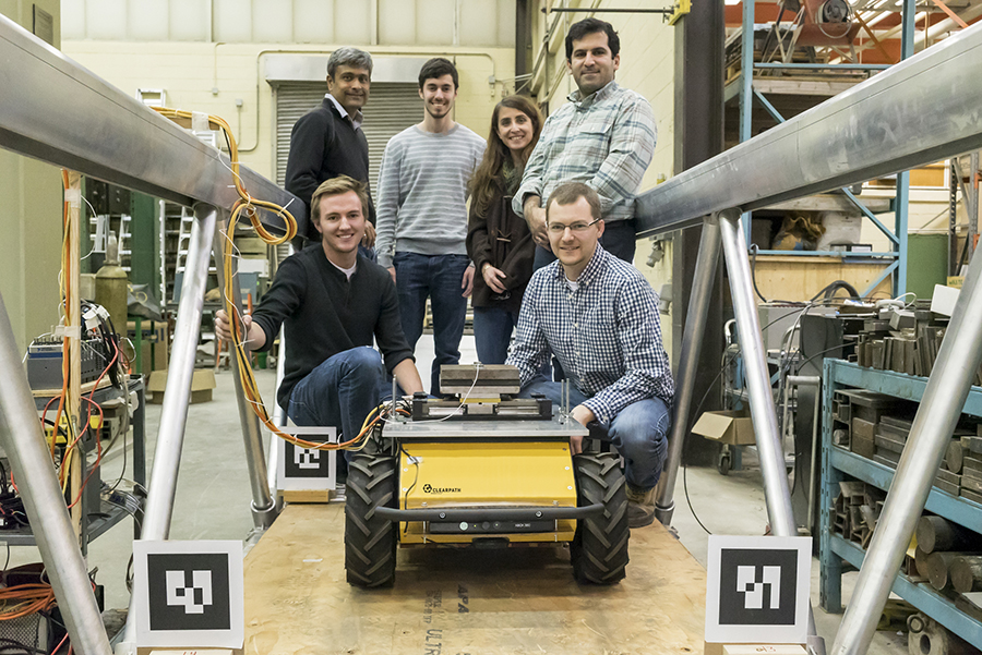
Amir Degani is an assistant professor at Technion Institute of Technology and Avi Kahnani is the CEO and Co-Founder of Israeli robotics start-up Fresh Fruits Robotics. Together, they are developing an apple harvesting robot that can autonomously navigate apple orchards and accurately pick fruit from the trees. I got the chance to sit down with Amir and Avi to learn more about the project. In our talk, they discussed the robot’s design, the challenges of apple picking, tree training and their experience demoing the robot for Microsoft’s CEO at the Think Next 2016 exhibition.

Tell me a little bit about CEAR Lab.

AD: I founded the CEAR Lab about four years ago after finishing my PhD and post doc at Carnegie Mellon University in Pittsburgh. I came back to the Technion in Israel and started the Civil, Environmental, Agricultural Robotics lab in the Faculty of Civil and Environmental Engineering. We work on soft robots, dynamic robots, and optimization of manipulators, mostly with civil applications, a lot of them related to agriculture. Other applications are search and rescue, automation in construction and environmental related work as well. But, generally, we’re mostly focused on agriculture robotics and robotic systems in the open field.

How did the apple harvesting robot project come to fruition?

AD: One of my PhD students is doing more theoretical work on task-based design of manipulators. Because cost is very important in agriculture, we’re trying to reduce price and find the optimal robot to do specific tasks. We’re actually seeing that different tasks, although they look very similar to us- apple picking or orange picking or peach picking – are actually very different if you look at the robot’s kinematics. We might need different joints, different lengths and so on. So we’re collecting data and modeling trees, we’re doing optimization and we’re finding the optimal robot for a specific task. This is something we have been working on for a few years. As part of this work, we are not only designing the optimal robot, but are also looking at designing the tree – finding the optimal tree in order to further simplify the robot.

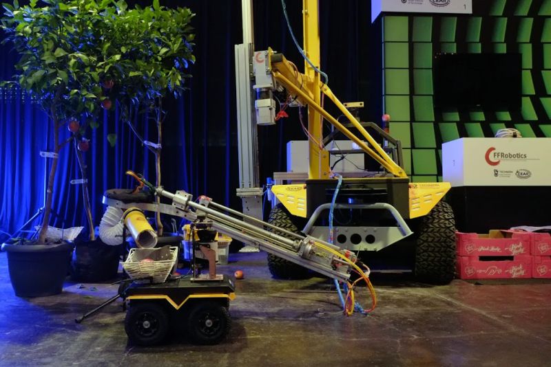
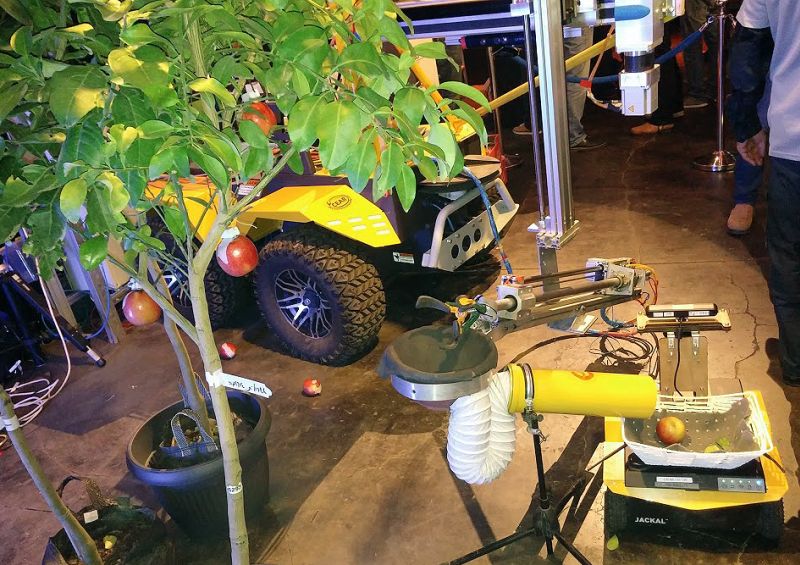
There is a new Israeli start-up called FFRobotics (Fresh Fruit Robotics or FFR). Avi, who is the CEO and Co-Founder, approached us a few years ago after hearing one of my students give a talk on optimization of a tasked-based harvesting manipulator. FFR are building a simple robotic arm – a three degree of freedom Cartesian robot, with the goal of having 8 or 12 of these arms picking apples (or other fruits) simultaneously. We were helping them with the arm’s optimization. We started collaborating and then a few months ago, Microsoft approached us and asked us to exhibit at their Think Next exhibition that they have every year. So we decided to put one of the arms on our Grizzly RUV robot which fit pretty nicely. We brought those to the demo, along with a few Jackals and had a pretty good time!

Tell me a bit about how the robot works and its components.

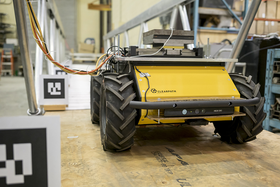
AD: So the FFR arm has a vision system to segment and detect the apples. After it finds an apple, it gives the controller the XYZ location and the arm then reaches for the fruit. It has an underactuated gripper at the end with a single motor which grips the apple and rotates it about 90 degrees to detach it. The arm doesn’t go back to the home position, it just retracts a bit, lets go and the apples go into a container. In our lab, we are concentrating right now on the automation of the mobile robots themselves – on the Grizzly, Husky, and Jackals – we have a few of your robots. Fruit Fresh Robotics is working primarily on the design of the manipulator.

What kind of vision sensors are being used?

AD: On the Grizzly, we have an IMU, SICK LIDAR in Front, a stereo camera on a Pant-Tilt unit, and a dGPS. The arm uses a Kinect to do the sensing, but FFR is also looking into time of flight sensors to provide better robustness in the field.

Robot prepares to pick the next apple off the tree at Microsoft’s Think Next exhibition. Source: Clearpath Robotics

What would you say is the most challenging part of automating apple picking?

AD: I believe that the most difficult thing is making something cheap and robust. I think the best way is to not only think of the robot but also to train the trees to be simpler. Now this has been done in the past decade or two to simplify human harvesting. In extreme cases, you can see fruiting walls that are nearly planar. They did this to make it a bit simpler for human harvesters. This is even more important for robotic harvesting. Trying to get a robot to harvest apples on a totally natural tree is extremely complex, and you will most likely need a 6-7 degree of freedom robot to do it. In terms of vision, perception will be very difficult. People have tried it in the past and it just doesn’t make sense and makes everything too expensive for farmers to use.

By taking simpler trees, ones that were trained and pruned as the ones in our collaboration with Fresh Fruit Robotics, you can actually use a three degree of freedom robot – the simplest Cartesian robot – to do the picking. But, I think you can even go further to make the tree in a more optimal shape for a robot, let’s say a quarter of a circle. This may not be good for a human, but might be perfect for a robot and perhaps will allow us to use simpler robots that only need two degrees of freedom. So, making the system robust while keeping costs down is the hardest part and in order to do that you have to work on the tree as well.

How exactly do you train a tree?

AD: Training systems such as a fruiting-wall require high density planting while ensuring that the trunk and branches are not too thick. In order to do that you have to support them with a trellis and other engineered support system. You want to make them optimal so that all the energy and water goes mostly to the fruit and not the tree itself. This has been done for a while now, and we are essentially piggy backing on that. The simplification of trees may be even more important for robotics than for humans, if we want robots to go into fruit picking and harvesting.

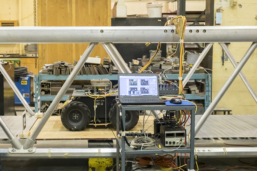
Can the robots autonomously navigate and patrol the apple orchards?

AD: Not at the moment. We are in the process of doing it now on all of our robots. Right now we are trying to do full SLAM on an orchard in order to do patrolling for harvesting. This is the goal we are aiming for this summer.

How do you compensate for weather effects?

AD: In Israel the weather is relatively mild, so the problem is usually with sun and wind rather than snow and rain. The main problem the weather creates is with the perception of the robot, having to compensate for changes in light and in position of the objects. To overcome this FFR uses a cover, like a tent, to shield the tree and the robot. If it’s windy, you have to use fast closed-loop control because if the target starts moving after it’s been perceived, the system has to keep on tracking it in order for the gripper to accurately grip the object where it is and not where it was 10 seconds ago.

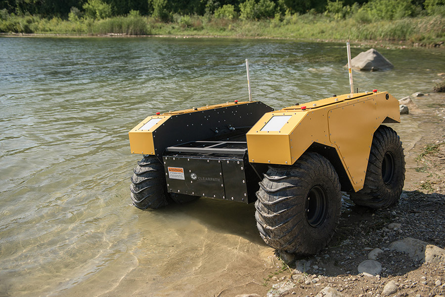
Why did you choose the Grizzly RUV for this project?

AD: We’ve had the Husky UGV for a while. We also have some older robots from 10 years ago, such as a tractor that we modified to be semi-autonomous. But, none of these vehicles were strong enough to actually do real work while being easily controllable. We wanted to carry bins full of fruit which weigh more than half a ton and we didn’t have a robot that could do that. Also, I wanted to have something that my students could take and apply the algorithms to a real-sized robot that could work in the field. We started with a TurtleBot to learn ROS, and then moved to the Husky. Then I wanted something I could just scale up and actually move to the field. That’s what we’re doing right now. It’s pretty new, so we’re in the early stages of working with it.

How did you find the integration process?

AD: Mechanical integration was very easy. We have not yet fully completed the electrical integration – instead we have two separate controllers and two separate electrical systems. Later on it will be relatively easy for the electrical system to be plugged into the robot since it uses the same voltage more or less. But right now it is decoupled.

Are you at a point where you can quantify the efficiency and cost benefits of the robots compared manual picking?

AK: We designed the system to pick approximately 10,000 high quality fruits per hour – that is without damaging the fruit while picking. Assuming working during the day only, the robot could potentially save farmers 25% in harvesting costs. It is important to understand that the same system will be able to pick other fresh fruits by replacing the end effector (gripper) and the software module. This option to harvest multiple fruits types increases the efficiency of the system dramatically.

What was it like to demo the robot to Satya Nadella, CEO of Microsoft, at the Think Next conference?

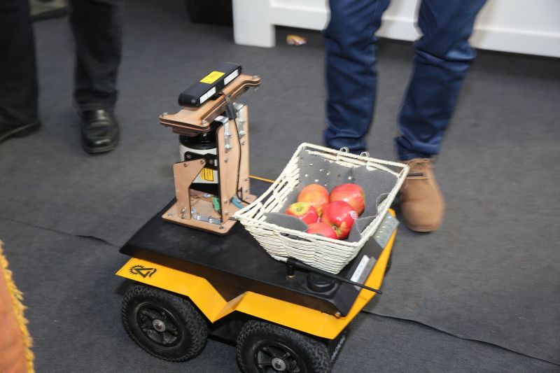
AD: It was exciting! He didn’t have a lot of time to spend at our booth. But it was an exciting exhibition with many demonstrators. We had the biggest robot for sure. It was fun! The FFR arm picked apples from the tree, and dropped them in the Jackal. Then, we drove the Jackal around delivering picked apples to people and they liked it. For safety reasons, we didn’t move the Grizzly. We just parked it and it didn’t move a centimeter the whole time. It was fun bringing such a big robot to the demo.

Picked apples were placed in a basket on top of a Jackal UGV and delivered to people in the crowd at Microsoft’s Think Next exhibition. Source: Clearpath Robotics

How close are you to a commercial release?

AK: Following last year’s field tests we believe the commercial system is about two years ahead. During the summer of 2016 we plan to test a full integrated system in the apple orchard, picking fruits from the trees all the way to the fruit bin. The first commercial system will be available for the 2017 apple picking season.

What is next for CEAR lab?

AD: We will continue working on the theoretical part of the optimization of the robotic arms. We’re looking into new ideas on re-configurability of arms – having arms doing different tasks and pretty easily switching from one task to another. With the Grizzly, we’re working on autonomous navigation of the apple orchards and are also working on a non-agricultural project related to search and rescue. We designed a suspension system on the Grizzly and mounted a stretcher on top of it. The motivation is to be able to evacuate wounded from harm’s way autonomously in rough terrain.

We are pretty happy with our robots. It’s a big family! We pretty much have all of Clearpath’s robots. Technical support is great and it’s been fun!

The post Interview: The Team Behind The Apple Harvesting Robot appeared first on Clearpath Robotics.


5 innovation challenges in materials transport

$
0
0

warehouse-distribution-centre-supply-chain

by: Meghan Hennessey

Walk into any manufacturing facility today. Forklifts and AGVs may be in operation serving specific parts of the manufacturing floor, but you’ll also see hundreds of people at work— pulling, tugging, and pushing goods from point A to point B. Why is it that we are still using humans — our most important asset — for materials transport? Yet, despite being the grease for the manufacturing wheel, materials transport remains an untapped opportunity for automation and innovation in most manufacturing establishments.

To continue to prosper and grow, manufacturers need to embrace innovation to overcome some of the significant challenges they face in the day-to-day operation of their business. Here are some of the challenges manufacturers are battling today:

Challenge #1: Adapting to a new velocity of change
From cola’s to custom cars, consumers are now demanding more variety in the goods they purchase. This insatiable appetite for choice is putting new pressure on industry to manufacture goods in a different way. To deal with the explosion of SKUs customers want available on store shelves, manufacturing environments need to be far more flexible than they’ve been in the past. To get there, manufacturers are turning to dynamic manufacturing methods such as mixed-model assembly lines (MMALs) and/or just-in-time (JIT) kit-based delivery to produce smaller batch runs with a greater variety and variation of products.

Challenge #2: Managing rising complexity

SKU proliferation is caused when consumers demand endless variations of a similar product. Source: usdagov/Flickr

Customers may demand that manufacturers produce a greater variety of product with a higher velocity, but these flexibility demands are creating chaos on the factory floor. As traditional automation and material handling systems are typically built into the infrastructure and cannot be easily or cost-effectively adapted to deal with ongoing change, manufacturers are continually struggling to contend with increasing complexity in the way products are built, the way raw materials are transported, and the way people and machines move through the facility.

Challenge #3: Remaining competitive on a global playing field
While North American manufacturers continue to wrestle with the complexities created by dynamic manufacturing models, there is yet another large dynamic at play: offshore competition. Manufacturers working in offshore locations such as China, Mexico, Eastern Europe and Africa are able to capitalize on lower local labor costs to produce goods and services for the market more affordably, making them significantly more competitive than their US counterparts. North American factory owners face higher real estate prices, higher labor costs, and more stringent environmental and regulatory compliance requirements than their offshore counterparts. Therefore, in order to be competitive in this global marketplace, a North American industrial center must find ways to be more efficient than its low cost country counterparts. Automation plays a significant role in helping North American manufacturers achieve operational parity; companies can optimize distribution, logistics, and production networks by using powerful data-processing and analysis capabilities.

Challenge #4: Reducing operating costs
In order to successfully compete against offshore rivals, US manufacturers need to reset the bar for production density and re-shore their operations. Automation is the linchpin within this strategy. As more manufacturers introduce automation, including robotics on the factory floor, production efficiency will rise, cost will fall, and the manufacturer will gain greater competitive advantage.

Challenge #5: Inefficient and chaotic materials transportation

Source: Flickr, creative commons

The variety and velocity at which goods must be produced, the increasing level of complexity this creates for manufacturers, and the ongoing cost pressures faced by North American industry become an acutely obvious problem when one looks at the way materials are transported and flow through a manufacturing facility. Three key elements tied to materials movement, transport (moving products that are not actually required to perform the processing), motion (people or equipment moving or walking more than is required to perform the processing) and waiting (for the next production step, interruptions of production during shift change) are among the original seven wastes of LEAN.

The post 5 Innovation Challenges in Materials Transport appeared first on Clearpath Robotics.

4 reasons why Industry 4.0 will leave AGVs behind

$
0
0
ATV in warehouse. Source: Wikipedia Commons
AGV in warehouse. Source: Wikipedia Commons

By Paula de Villavicencio

Technology has been in development for the last decade and has now come to fruition in the form of self-driving vehicles. These vehicles are driving into industrial centers and beginning to replace traditional AGVs, and it’s no wonder why. The first AGV was introduced in the early 1950s and more than 50 years later it has marginally advanced from following radio transmissions from the ceiling to following magnetic tape on the floor. Its slow advancement isn’t the only limitation; AGVS are fixed, reactive, captured and adoptive machines, and they leave a lot to be desired in today’s complex manufacturing environment.

AGV_BlogPost

1. Fixed not flexible
Like trains on their tracks, AGVs are fixed to a certain pathway and are unable to move off of it. These are not flexible machines, and while repeatable point-to-point navigation tasks are possible, many companies have fork trucks and manually driven tug vehicles working alongside the AGVs. Dynamic pathways are a necessary evolution in Industry 4.0, especially for innovating manufacturers with complex production systems.

2. Reactive not proactive
Yet, unlike trains, AGVs cannot move onto a new track direction to avoid collision or change their direction. In fact, if an AGV breaks down while on a preprogrammed pathway, all AGVs following the same pathway cannot move around it, and are unable to deliver or pick up their loads. This loss in movement can cost a company a great deal of money in a short amount of time.

3. Captured not collaborative
These machines are also unable to collaborate amongst each other to share the work in the most efficient way possible. Those AGVs that are preprogrammed to a specific pathway cannot move to a different path rapidly or easily to perform a different job. They are held captive in their preprogrammed task regardless of efficiency or changing manufacturing needs.

4. Adoptive not adaptive
Since the preprogrammed pathways have to be simple and unobstructed for the AGVs, many facilities pre-plan their layouts with the machines in mind. Transport aisles are designed for isolated AGV paths, and work areas are laid out to accommodate the vehicles’ planned route. When it comes to AGVs, manufacturers have to adapt to the machines, instead of the AGVs incorporating into an already existing facility. In some cases, factories and warehouses resort to manual transport methods instead of adopting AGV technology and all the prerequisite planning that it requires.

By advancing material transport for Industry 4.0 capabilities, we will see more technologies take the factory floor. Self-driving vehicles can offer flexibility, proactive planning, collaboration, and adaptive behaviours.

Interview: International Ground Vehicle Ground Competition (IGVC) winner on “Bigfoot 2” Husky UGV

$
0
0
Photo credit: Lawrence Tech University IGVC Facebook

By: Chris Bogdon

The International Ground Vehicle Ground Competition (IGVC) is an annual event that brings together teams of college students from all over the globe to compete in an autonomous ground vehicle competition. Teams are tasked to design and construct a fully autonomous unmanned robotic vehicle that can navigate around a challenging outdoor obstacle course under a prescribed time. This year’s IGVC went down in June at Oakland University, and while the competition was stiff, only one team could come out on top. That team was Lawrence Teach University (LTU), whose robot, Bigfoot 2, was built using the Husky UGV robotic platform.

We had a chance to sit down for a quick Q&A with team captain, Gordon Stein, to learn more about the design of the robot, challenges and key lessons learned by taking part in the competition.

Q: Tell us a bit about the design of Bigfoot 2?

A: Bigfoot 2 uses the Clearpath Husky platform, with our own frame and electronics placed on top of it. For sensors, we have a 2D LIDAR, a camera, a GPS, and a compass. The computer we used was one of the laptops our school provides to students. This meant we could easily get a replacement if needed. Our software is made in C#, which makes it easier for students in the robotics programming course to join the team.

We modified the platform to have larger tires with a smoother tread. The original tires had too much traction, and we were afraid that we would get disqualified from them ripping up the turf at the competition. In addition, it makes it easier for the robot to turn in place, and made the robot able to go slightly faster.

Photo credit: Lawrence Tech University IGVC Facebook

Q: Why did you choose the Husky UGV as your mobile base over other mobile platforms or creating your own?

A: Our team’s philosophy was to use as many “off-the-shelf” components as possible. We represent the Computer Science department, so we wanted to spend as much time as possible on our programming. Using an existing platform allowed us to have a working robot earlier in the year, so we could start programming instead of waiting for the chassis to be assembled.

Q: What was the most challenging part of preparing for the competition?

A: The most challenging part is testing. Our team has a simulator we made in a previous year, and we had set up a practice course on campus, but we still couldn’t prepare for everything at the competition. This is especially difficult because we don’t know the obstacles ahead of time. In the previous year, we didn’t prepare for ramps and a ramp stopped us. This year, we tested to make sure it could go over ramps and no ramps were at the competition. The advanced course always has obstacles that none of the teams are ready for, and that’s part of the challenge.

Q: What aspect of the design were you most and least worried going into the competition?

A: We were most worried about waterproofing. Our team tradition for the past few years had been to just attach an umbrella to the robot, but this doesn’t win us any points with the judges, and it doesn’t let us run in serious rain. The Husky chassis is water resistant, but the electronics we had on top of it is not. We purchased some vinyl material to use for waterproofing, but we weren’t able to make it into a real cover in time.

We were least worried about the new tires. We tested them to make sure they would work on slopes and ramps, and they definitely improved the steering.

Photo credit: Lawrence Tech University IGVC Facebook

Q: What were the key lessons learned by participating in the IGVC competition?

A: The key lesson we learned was to keep things simple. Some of the teams had very elaborate sensors and relied on dozens of ROS packages for their code, and many of them seemed to be having issues at the competition. While a 3D LIDAR would’ve opened up some new possibilities, we only needed a 2D LIDAR to see the barrels.

Q: What advice would you give to teams participating in next year’s challenge?

A: Our advice would be to spend time trying new ideas. We had one team member whose job was to try new ways to automatically adjust our camera to changing lighting conditions. None of them ended up being used at the competition, but it still allowed us to see what possible other solutions there could be.

See Bigfoot 2 in action

Watch Bigfoot 2 navigate the Auto-Nav Challenge Advanced Course

The post Interview: IGVC Winner on “Bigfoot 2” Husky UGV appeared first on Clearpath Robotics.

Clearpath Robotics launches “Warthog UGV”, the amphibious robot

$
0
0

warthog-UGV

Clearpath Robotics, a leading provider of mobile robotic platforms for research and development, has partnered with ARGO XTR to release Warthog – a large, amphibious, all-terrain mobile robot designed for application development. Warthog enables researchers to reliably test, validate, and advance their robotics research faster than ever before in real-world conditions, whether on land or in water.

“ARGO XTR (Xtreme Terrain Robotics) has a terrific record of manufacturing rock-solid outdoor platforms,” says Julian Ware, General Manager for Research Solutions at Clearpath Robotics. “Combined with our expertise in robotics, we’ve developed rugged platform suitable for a wide range of robotics applications in mining, agriculture, forestry, space, and environmental monitoring.”

Warthog’s light-weight aluminum chassis, low ground pressure, passive suspension system, and 24” traction tires allow it to easily traverse a variety of tough terrains including soft soils, thick muds and steep grades, all while carrying up to 272 kg of payload.    With built-in bilge pumps and an IP rating of 67, Warthog is fully weather-proof and amphibious, capable of moving through deep waterways at up to 4 km/h, or travel at speeds of up to 18 km/h while on land. The all-electric, skid steer platform has expandable power allowing for a runtime of 6 hrs and can be outfitted with quad tracks for ultimate traction and maneuverability in snow and sand.

“ARGO XTR is excited to partner with a progressive robotics company like Clearpath with our platform,” says Jason Scheib, ARGO XTR Robotics Program Director.  “The combination of our proven experience in amphibious and extreme terrain environments with our platforms with the progressive software and sensor integration from Clearpath Robotics, has created a second to none solution for a myriad of research and commercial applications.”

Designed for end-to-end integration and customization, Warthog includes an internal computer, IMU, wheel encoders, and mounting racks, as well as accessible user power and communication ports for integrating sensors, manipulators, and other third-party hardware.   Warthog is shipped with the Robot Operating System (ROS) preconfigured and a Gazebo simulation model, allowing researchers to get started quickly with existing research and widely available open-source ROS libraries.

Click here for more information.

If you liked this article, you may also be interested in:

See all the latest robotics news on Robohub, or sign up for our weekly newsletter.

Customer story: Deployable, autonomous vibration control of bridges using Husky UGV

$
0
0
Image: Clearpath
Image: Clearpath

Sriram Narasimhan’s research team are shaking things up in the Civil Engineering Structures Lab at the University of Waterloo. The research, which is led by Ph.D Candidate Kevin Goorts, is developing a new mobile damping system for suppressing unwanted vibrations in lightweight, flexible bridges. Whereas damping systems are often permanent fixtures built into the bridge, their system is designed to be adaptable, autonomous, and better suited for rapid, temporary deployment.

A SHIFT TOWARDS FLEXIBLE, LIGHT-WEIGHT STRUCTURES

Their work follows a recent industry shift towards using lightweight materials in the construction of civil engineering structures. Driven primarily by cost savings, as well as both the ease and speed of deployment, these lightweight structures could be a pedestrian bridge or a temporary bridge used in disaster relief scenarios, and are often more sensitive to external forces due to the reduced self-weight, and therefore require auxiliary damping devices.

Husky-based mobile bridge damping system on a full-scale aluminum pedestrian bridge. Image: Clearpath

HUSKY UGV: THE IDEAL MOBILE ROBOTIC PLATFORM

At the center of the team’s mobile control system is a Husky unmanned ground vehicle (UGV). An electromechanical mass damper mounted on top of the Husky is used to generate inertial control forces which are magnified by the body dynamics of the Husky. When situated on a bridge, the system is able to respond to changes in the structural response by autonomously positioning itself at the appropriate location and applying the desired control force.

For Goorts’ research, Husky UGV was the ideal mobile base upon which to develop their system. “The Husky is a rugged vehicle suitable for outdoor applications with sufficient payload capacity for both the damper and associated computational equipment.” said Goorts. “The low-profile and large lug thread tires are well suited for providing the necessary static friction to prevent sliding and transfer control forces. Moreover, Husky’s readily available ROS (Robot Operating System) integration allowed us to use several sensor types and position control algorithms.”

Linear motor and front-facing Kinect vision sensor mounted on Husky UGV mobile base. Image: Clearpath

The Husky is also equipped with a laptop running ROS and Kinect vision sensors on the front and back of the vehicle. Using wheel encoder data and measurements from the Kinect sensors, the system is able to perform SLAM (Simultaneous Localization and Mapping) and autonomously navigate back and forth along the span of the bridge. One of the immediate challenges the team faced was getting the robot to accurately localize on a bridge with a repetitive structural design – everything looked the same to the robot from different positions. To overcome this, they placed unique AR (augmented reality) tags along the bridge between which the robot could navigate.

A National Instruments (NI) cRIO is being used for all data processing tasks and execution of the structural control loops, and a TCP data link communicates between the ROS laptop and cRIO. Image: Clearpath.

BRIDGE VIBRATIONS REDUCED BY 70%

The effectiveness of the control system is tested using real-time hybrid simulation (RTHS), a dynamic testing method that couples the physical control system with a numerical model of the structure. These tests were carried out on a full-scale aluminum pedestrian bridge with re-designed panels to measure the forces being applied by the system. Results from the simulations show the system can provide up to a 70% reduction in the lateral displacement of the bridge.

The current prototype is suitable for bridges with a mass up to 1-tonne and is scalable to accommodate larger structures, either with a larger vehicle or with multiple vehicles that work cooperatively. Looking forward, the team is exploring the idea of making the system vehicle agnostic, which could allow any vehicle to be turned into an autonomous bridge stabilizing machine.

The post Customer Story: Deployable, Autonomous Vibration Control of Bridges Using Husky UGV appeared first on Clearpath Robotics.

If you liked this article, you may also be interested in:

See all the latest robotics news on Robohub, or sign up for our weekly newsletter.

Rapid outdoor/indoor 3D mapping with a Husky UGV

$
0
0

by Nicholas Charron

The need for fast, accurate 3D mapping solutions has quickly become a reality for many industries wanting to adopt new technologies in AI and automation. New applications requiring these 3D mapping platforms include surveillance, mining, automated measurement & inspection, construction management & decommissioning, and photo-realistic rendering. Here at Clearpath Robotics, we decided to team up with Mandala Robotics to show how easily you can implement 3D mapping on a Clearpath robot.

3D Mapping Overview

3D mapping on a mobile robot requires Simultaneous Localization and Mapping (SLAM), for which there are many different solutions available. Localization can be achieved by fusing many different types of pose estimates. Pose estimation can be done using combinations of GPS measurements, wheel encoders, inertial measurement units, 2D or 3D scan registration, optical flow, visual feature tracking and others techniques. Mapping can be done simultaneously using the lidars and cameras that are used for scan registration and for visual position tracking, respectively. This allows a mobile robot to track its position while creating a map of the environment. Choosing which SLAM solution to use is highly dependent on the application and the environment to be mapped. Although many 3D SLAM software packages exist and cannot all be discussed here, there are few 3D mapping hardware platforms that offer full end-to-end 3D reconstruction on a mobile platform.

Existing 3D Mapping Platforms

We will briefly highlight some more popular alternatives of commercialized 3D mapping platforms that have one or many lidars, and in some cases optical cameras, for point cloud data collection. It is important to note that there are two ways to collect a 3D point cloud using lidars:

1. Use a 3D lidar which consists of one device with multiple stacked horizontally laser beams
2. Tilt or rotate a 2D lidar to get 3D coverage

Tilting of a 2D lidar typically refers to back-and-forth rotating of the lidar about its horizontal plane, while rotating usually refers to continuous 360 degree rotation of a vertically or horizontally mounted lidar.

Example 3D Mapping Platforms: 1. MultiSense SL (Left) by Carnegie Robotics, 2. 3DLS-K (Middle) by Fraunhofer IAIS Institute, 3. Cartographer Backpack (Right) by Google.

1. MultiSense SL

The MultiSense SL was developed by Carnegie Robotics and provides a compact and lightweight 3D data collection unit for researchers. The unit has a tilting Hokuyo 2D lidar, a stereo camera, LED lights, and is pre-calibrated for the user. This allows for the generation of coloured point clouds. This platform comes with a full software development kit (SDK), open source ROS software, and is the sensor of choice for the DARPA Robotics Challenge for humanoid robots.

2. 3DLS-K

The 3DLS-K is a dual-tilting unit made by Fraunhofer IAIS Institute with the option of using SICK LMS-200 or LMS-291 lidars. Fraunhofer IAIS also offers other configurations with continuously rotating 2D SICK or Hokuyo lidars. These systems allow for the collection of non-coloured point clouds. With the purchase of these units, a full application program interface (API) is available for configuring the system and collecting data.

3. Cartographer Backpack

The Cartographer Backpack is a mapping unit with two static Hokuyo lidars (one horizontal and one vertical) and an on-board computer. Google released cartographer software as an open source library for performing 3D mapping with multiple possible sensor configurations. The Cartographer Backpack is an example of a possible configuration to map with this software. Cartographer allows for integration of multiple 2D lidars, 3D lidars, IMU and cameras, and is also fully supported in ROS. Datasets are also publicly available for those who want to see mapping results in ROS.

Mandala Mapping – System Overview

Thanks to the team at Mandala Robotics, we got our hands on one of their 3D mapping units to try some mapping on our own. This unit consists of a mount for a rotating vertical lidar, a fixed horizontal lidar, as well as an onboard computer with an Nvidia GeForce GTX 1050 Ti GPU. The horizontal lidar allows for the implementation of 2D scan registration as well as 2D mapping and obstacle avoidance. The vertical rotating lidar is used for acquiring the 3D point cloud data. In our implementation, real-time SLAM was performed solely using 3D scan registration (more on this later) specifically programmed for full utilization of the onboard GPU. The software used to implement this mapping can be found on the mandala-mapping github repository.

Scan registration is the process of combining (or stitching) together two subsequent point clouds (either in 2D or 3D) to estimate the change in pose between the scans. This results in motion estimates to be used in SLAM and also allows a new point cloud to be added to an existing in order to build a map. This process is achieved by running iterative closest point (ICP) between the two subsequent scans. ICP performs a closest neighbour search to match all points from the reference scan to a point on the new scan. Subsequently, optimization is performed to find rotation and translation matrices that minimise the distance between the closest neighbours. By iterating this process, the result converges to the true rotation and translation that the robot underwent between the two scans. This is the process that was used for 3D mapping in the following demo.

Mandala Robotics has also released additional examples of GPU computing tasks useful for robotics and SLAM. These examples can be found here.

Mandala Mapping Results

The following video shows some of our results from mapping areas within the Clearpath office, lab and parking lot. The datasets collected for this video can be downloaded here.

The Mandala Mapping software was very easy to get up and running for someone with basic knowledge in ROS. There is one launch file which runs the Husky base software as well as the 3D mapping. Initiating each scan can be done by sending a simple scan request message to the mapping node, or by pressing one button on the joystick used to drive the Husky. Furthermore, with a little more ROS knowledge, it is easy to incorporate autonomy into the 3D mapping. Our forked repository shows how a short C++ script can be written to enable constant scan intervals while navigating in a straight line. Alternatively, one could easily incorporate 2D SLAM such as gmapping together with the move_base package in order to give specific scanning goals within a map.

Why use Mandala Mapping on your robot?

If you are looking for a quick and easy way to collect 3D point clouds, with the versatility to use multiple lidar types, then this system is a great choice. The hardware work involved with setting up the unit is minimal and well documented, and it is preconfigured to work with your Clearpath Husky. Therefore, you can be up and running with ROS in a few days! The mapping is done in real time, with only a little lag time as your point cloud size grows, and it allows you to visualize your map as you drive.

The downside to this system, compared to the MultiSense SL for example, is that you cannot yet get a coloured point cloud since no cameras have been integrated into this system. However, Mandala Robotics is currently in the beta testing stage for a similar system with an additional 360 degree camera. This system uses the Ladybug5 and will allow RGB colour to be mapped to each of the point cloud elements. Keep an eye out for a future Clearpath blogs in case we get our hands on one of these systems! All things considered, the Mandala Mapping kit offers a great alternative to the other units aforementioned and fills many of the gaps in functionality of these systems.

The post Rapid Outdoor/Indoor 3D Mapping with a Husky UGV appeared first on Clearpath Robotics.

ROS 101: Drive a Husky!

$
0
0

ROS101_Clearpath

In the previous ROS 101 post, we showed how easy it is to get ROS going inside a virtual machine, publish topics and subscribe to them. If you haven’t had a chance to check the out all the previous ROS 101 tutorials, you may want to do so before we go on. In this post, we’re going to drive a Husky in a virtual environment, and examine how ROS passes topics around.

An updated version of the Learn_ROS disk is available here:

https://s3.amazonaws.com/CPR_PUBLIC/LEARN_ROS/Learn_ROS-disk1.vmdk
https://s3.amazonaws.com/CPR_PUBLIC/LEARN_ROS/Learn_ROS.ovf

Login (username): user
Password: learn

If you just downloaded the updated version above, please skip the next section. If you have already downloaded it, or are starting from a base install of ROS, please follow the next section.

Updating the Virtual Machine

Open a terminal window (Ctrl + Alt + T), and enter the following:

sudo apt-get update
sudo apt-get install ros-hydro-husky-desktop

Running a virtual Husky

Open a terminal window, and enter:

roslaunch husky_gazebo husky_empty_world.launch

Open another terminal window, and enter:

roslaunch husky_viz view_robot.launch

You should be given two windows, both showing a yellow, rugged robot (the Husky!)

Screenshot-from-2014-03-14-07_34_30


The first window shown is Gazebo. This is where we get a realistic simulation of our robot, including wheel slippage, skidding, and inertia. We can add objects to this simulation, such as the cube above, or even entire maps of real places.

Screenshot-from-2014-03-14-07_35_36

The second window is RViz. This tool allows us to see sensor data from a robot, and give it commands (We’ll talk about how to do this in a future post). RViz is a more simplified simulation in the interest of speed.

We can now command the robot to go forwards. Open a terminal window, and enter:

rostopic pub /husky/cmd_vel geometry_msgs/Twist -r 100 '[0.5,0,0]' '[0,0,0]'

In the above command, we publish to the /husky/cmd_vel topic, of topic type geometry_msgs/Twist, at a rate of 100Hz. The data we publish tells the simulated Husky to go forwards at 0.5m/s, without any rotation. You should see your Husky move forwards. In the gazebo window, you might notice simulated wheel slip, and skidding.

Using rqt_graph

We can also see the structure of how topics are passed around the system. Leave the publishing window running, and open a terminal window. Type in:

rosrun rqt_graph rqt_graph

This command generates a representation of how the nodes and topics running on the current ROS Master are related. You should get something similar to the following:

Screenshot-from-2014-03-14-08_10_25


The highlighted node and arrow show the topic that you are publishing to the simulated Husky. This Husky then goes on to update the gazebo virtual environment, which takes care of movement of the joints (wheels) and the physics of the robot. The rqt_graph command is very handy to use, when you are unsure who is publishing to what in ROS. Once you figure out what topic you are interested in, you can see the content of the topic using rostopic echo.

Using tf

In Ros, tf is a special topic that keeps track of coordinate frames, and how they relate to each other. So, our simulated Husky starts at (0,0,0) in the world coordinate frame. When the Husky moves, it’s own coordinate frame changes. Each wheel has a coordinate frame that tracks how it is rotating, and where it is. Generally, anything on the robot that is not fixed in space, will have a tf describing it. In the rqt_graph section, you can see that the /tf topic is published to and subscribed from by many different nodes.

One intuitive way to see how the tf topic is structured for a robot is to use the view_frames tool provided by ROS. Open a terminal window. Type in:

rosrun tf2_tools view_frames.py

Wait for this to complete, and then type in:

evince frames.pdf

This will bring up the following image.

Screenshot-from-2014-03-18-12_20_59Here we can see that all four wheel are referenced to the base_link, which is referenced from the base_frootprint. (Toe bone connected to the foot bone, the foot bone….). We also see that the odom topic is driving the reference of the whole robot. This means that if you write to the odom topic (IE, when you publish to the /cmd_vel topic) then the whole robot will move.


Tweet to drive a robot!

$
0
0

tweetbot

Happy Birthday!! Clearpath is officially 5 years old and what better way to celebrate than let all of our fans drive a robot. No matter where you are in the world, you can experience what it’s like to drive Husky – well, a very mini, hacked-together Husky that is. We’ve put together ‘twit-bot’ for your enjoyment so you can move our bot around all from the convenience of your smartphone using Twitter.

Here’s how it works:

Step 1: Mention Clearpath’s Twitter handle (@ClearpathRobots)
Step 2: Hash tag #MoveRobot
Step 3: Write the action you’d like it to take (examples are below)
Step 4: Watch it move on the live feed: http://www.twitch.tv/twitbot_cpr
Step 5: Share with your friends!

How does it move?

This little twit-bot can go just about anywhere and in any direction using the commands below (case insensitive).  The delay between the tweet and the streaming is about 30 seconds:

  • “forward” or “fwd”
  • “backward” or “bck”
  • “right” or “rght”
  • “left” or “ft”
  • “stop” or “stp”

You can also tweet colors to change the colors of the LED lights: blue, red, white, etc.

Of course, there are some hidden key words – easter eggs – in there too that you’ll just have to figure out on your own. I wonder if pop-a-wheelie is on the list?…

If you liked this article, you may also be interested in Clearpath’s ROS 101 Tutorials:

See all the latest robotics news on Robohub, or sign up for our weekly newsletter.

ROS 101: Drive a Grizzly!

$
0
0

ROS101_logo

So you have had a taste of driving a virtual Husky in our previous tutorial, but now want to try something a little bigger? How about 2000 lbs bigger?

Read on to learn how to drive a (virtual) Grizzly, Clearpath Robotic’s largest and meanest platform. If you are totally new to ROS, be sure to check out our tutorial series starting here and the ROS Cheat Sheet. Here is your next ROS 101 dose.

An updated version of the Learn_ROS disk is available here:

https://s3.amazonaws.com/CPR_PUBLIC/LEARN_ROS/Learn_ROS-disk1.vmdk
https://s3.amazonaws.com/CPR_PUBLIC/LEARN_ROS/Learn_ROS.ovf

Login (username): user
Password: learn

Updating the Virtual Machine

Open a terminal window (Ctrl + Alt + T), and enter the following:

sudo apt-get update
sudo apt-get install ros-hydro-grizzly-simulator 
sudo apt-get install ros-hydro-grizzly-desktop 
sudo apt-get install ros-hydro-grizzly-navigation

Running a virtual Grizzly

Open a terminal window, and enter:

roslaunch grizzly_gazebo grizzly_empty_world.launch

Open another terminal window, and enter:

roslaunch grizzly_viz view_robot.launch

You should be given two windows, both showing a yellow, rugged robot (the Grizzly!). The left one shown is Gazebo. This is where we get a realistic simulation of our robot, including wheel slippage, skidding, and inertia. We can add objects to this simulation, or even entire maps of real places.

Grizzly_gazebo-2

Grizzly RUV in simulation

The right window is RViz. This tool allows us to see sensor data from a robot, and give it commands (in a future post). RViz is a more simplified simulation in the interest of speed.

Grizzly_rviz

RViz – sensor data

We can now command the robot to go forwards. Open a terminal window, and enter:

rostopic pub /cmd_vel geometry_msgs/Twist -r 100 '[0.5,0,0]' '[0,0,0]'

In the above command, we publish to the cmd_vel topic, of topic type geometry_msgs/Twist, at a rate of 100Hz. The data we publish tells the simulated Grizzly to go forwards at 0.5m/s, without any rotation. You should see your Grizzly move forwards. In the gazebo window, you might also notice simulated wheel slip, and skidding. Enjoy and stay tuned for more soon!


See all the ROS101 tutorials here. If you liked this article, you may also be interested in:

See all the latest robotics news on Robohub, or sign up for our weekly newsletter.

Grizzly on the Mars Emulation Terrain at NCFRN

$
0
0

ncfrnblog3

by Ryan Gariepy

I recently spent over a week in Montreal talking with – and learning from – the Canadian field robotics community, first at the Computer and Robot Vision (CRV) conference and then at the NCFRN Field Trials. This was my first time attending CRV since I spoke at the 2012 conference in Toronto, and it’s quite inspiring how much robotics is spreading throughout Canada. Keynote speakers were Raff D’Andrea from ETH-Z and Frank Dellaert from Georgia Tech, both of whom had excellent talks. Bonus points to Frank for pointing out factor graphs to me for the first time, and Raff for bringing the best tabletop demo ever!

ncfrnblog4

Testing out new software algorithms on Kingfisher

CRV transitioned right into the opening meetings of the NCFRN Field Trials. Or, for those of you who don’t like nested acronyms, the National Science and Engineering Research Council Canadian Field Robotics Network Field Trials. The NCFRN makes up Canada’s leading field robotics researchers, companies, and supporting government organizations, and has just marked its second year in existence. The first two days are filled with presentations, seminars, and poster sessions, and from there it’s into the eponymous field. Something which was both surprising and inspiring for me was seeing that Clearpath hardware represented every single ground vehicle and surface vessel in the poster session.

Spread from the Mars Emulation Terrain at the Canadian Space Agency to the east (aka, the “Mars Yard”) to the McGill MacDonald campus to the west, the field trials were quite the experience. Researchers and partners were able to see the algorithms operating live. They were able to collaborate on combining their technologies, and, in the most extreme cases, swapped code between robots to test how robust their approaches were. In my opinion, one of the most valuable aspects of the field trials is improving how testing and deploying autonomous vehicles in remote locations is completed. Teams’ preparations ranged from being as minimal and lightweight as possible to turning an entire cube van into a remote lab.

This years’ field trials also mark an important milestone for Clearpath Robotics: It’s the first time we’ve seen someone make coffee using our robots (at least, the first time we’re aware of it). Apparently it’s easier to plug a coffee maker into a Grizzly than it is to run an extension cord. I can understand why they were making coffee; this was the ASRL team which did 26 repeated traverses of nearly a kilometer each based on a single, visually taught route. And, since the ASRL has a thing for setting videos of our robots to music, here’s the research set to music.

ncfrnblog5

Taking Husky for a walk in Montreal at NCFRN

I’ll close off by sharing the kind of experience which keeps us going: On the last day of the trials, I could only see six robots left rolling around the Mars Yard. There were three kinds, and all were robots designed and built by the Clearpath team – we’re thrilled to see that our work is having an impact on the robotics community and we can’t wait to see how Year 3 Trials will go next spring!

Clearpath introduces Jackal, their new unmanned ground vehicle

$
0
0

We’ve been keeping a huge secret and now we’re ready to share it… Earlier this year, Army Research Labs (ARL) contracted us to design an affordable, portable research platform for outdoor use. Working with them during the development phase, their team provided feedback for iteration on the platform’s performance and capabilities. And now, it’s ready to release to the world. Introducing the newest addition to Clearpath’s black and yellow robot family: Jackal Unmanned Ground Vehicle!

Jackal offers end-to-end integration including a built-in GPS, IMU, and computer, and a configurable top-plate. Engineered for the great outdoors, Jackal’s sturdy metal chassis, weatherproof design (IP 62) and skid-steer drive enables all-terrain operation, as well as lab experimentation, for a variety of applications.

Read more on Clearpath Robotics Inc.

ROS 101: Creating a publisher node

$
0
0

ROS101_logo

By Martin Cote

In our previous post, we graduated from driving a Husky to taking on a Grizzly! Now it’s time to get down and dirty with what ROS is really made of: nodes! We will first be creating a workspace to work from, then we will write a simple publisher that will make our virtual Husky drive around randomly. If this is your first time visiting a Clearpath Robotics ROS 101 blog, get started here.

Creating a workspace and package

Before we begin writing a node, we need to create a workspace and a package. Workspaces are simply directories to store all of your packages. First we will need to create a new directory.

mkdir ~/ros101

This created a directory in your home folder, which we will use as a workspace directory. We now need to create a subdirectory in your workspace directory to store all your source code for your packages.

mkdir ~/ros101/src

The last step to creating the workspace will be to initialize the workspace with catkin_init_workspace.

cd ~/ros101/src
catkin_init_workspace

Now that our workspace has been created, we will create a package in the src directory we just created. This can be done by navigating to the ~/ros101/src directory, which you should have already done in the last step, and using the catkin_create_pkg command  followed by what we want the package to be named, and then followed by what other packages our package will be dependent on; this command creates another directory for your new package, and two new configuration files inside that directory with some default settings.

catkin_create_pkg random_husky_driver roscpp std_msgs

You can see that this created CMakeLists.txt and package.xml inside the random_husky_driver directory; this is also where you will store all your source code for your packages. The roscpp and std_msgs  dependencies were added into the CMakeLIst.txt and package.xml.

Writing the publisher

As mentioned in our previous post, a publisher publishes messages to a particular topic. For this tutorial, we will be publishing random commands to the /husky/cmd_vel topic to make your Husky visualization drive itself. Start by creating a file in your ~/ros101/src/random_husky_driver directory called random_driver.cpp, and copy the following code.

#include <ros/ros.h>
#include <geometry_msgs/Twist.h> 
#include <stdlib.h> 

int main(int argc, char **argv) {
     //Initializes ROS, and sets up a node
     ros::init(argc, argv, "random_husky_commands");
     ros::NodeHandle nh;

     //Ceates the publisher, and tells it to publish
     //to the husky/cmd_vel topic, with a queue size of 100
     ros::Publisher pub=nh.advertise<geometry_msgs::Twist>("husky/cmd_vel", 100);

     //Sets up the random number generator
     srand(time(0));

     //Sets the loop to publish at a rate of 10Hz
     ros::Rate rate(10);

       while(ros::ok()) {
            //Declares the message to be sent
            geometry_msgs::Twist msg;
           //Random x value between -2 and 2
           msg.linear.x=4*double(rand())/double(RAND_MAX)-2;
           //Random y value between -3 and 3
           msg.angular.z=6*double(rand())/double(RAND_MAX)-3;
           //Publish the message
           pub.publish(msg);

          //Delays untill it is time to send another message
          rate.sleep();
         }
}

Let’s break down this code line by line:

#include <ros/ros.h>
#include <geometry_msgs/Twist.h> 

These lines includes the headers that we are going to need. The <ros/ros.h> header is required for ROS functionality and the <geometry_msgs/Twist.h> is added so that we can create a message of that type.

ros::init(argc, argv, "random_husky_commands");
ros::NodeHandle nh;

The first line, ros::init,  is used to initialize the ROS node, and name it “random_husky_commands”, while ros:NodeHandle starts the node.

ros::Publisher pub=nh.advertise<geometry_msgs::Twist>("husky/cmd_vel", 100);

Publishing a message is done using ros:Publisher pub=nh.advertise, followed by the message type that we are going to be sending, in this case it is a geometry_msga::Twist, and the topic that we are going to be sending it too, which for us is husky/cmd_vel.

The 100 is the message queue size; that is, if you are publishing message faster than what roscpp can send, 100 messages will be saved in the queue to be sent. The larger the queue, the more delay in robot movement in case of buffering.

Therefore in a real life example, you will want to have a smaller queue in the case of robot movement, where delay in movement commands are undesirable and even dangerous, but dropped messages are acceptable. In the case of sensors, it is recommended to use a larger queue, since delay is acceptable to ensure no data is lost.

ros::Rate rate(10)
...
rate.sleep()

ROS is able to control the loop frequency  using ros:Rate to dictate how rapidly the loop will run in Hz. rate.sleep will delay a variable amount of time such that your loop cycles at the desired frequency. This accounts for time consumed by other parts of the loop. All Clearpath robots require a minimum loop rate of 10Hz.

while(ros::ok())

The ros::ok function will return true unless it receives a command to shut down, either by using the rosnode kill command, or by the user pusing Ctrl-C in a terminal.

geometry_msgs::Twist msg;

This creates the message we are going to send, msg, of the type geometry_msgs:Twist
msg.linear.x=4*double(rand())/double(RAND_MAX)-2;
msg.angular.z=6*double(rand())/double(RAND_MAX)-3;

Screen-Shot-2014-09-19-at-10.16.36-AM-300x151

These lines calculate the random linear x and angular z values that will be sent to Husky.

pub.publish(msg)

We are finally ready to publish the message! The pub.publish adds msg to the publisher queue to be sent.

Compiling the random Husky driver

Compilation in ROS in handled by the catkin build system. The first step would usually be to set up our package dependencies in the CMakeLists.txt and package.xml. However this has already been done for us when we created the package and specified our dependencies. The next step is then to declare our new node as a executable, this is done by adding the following two lines to the CMakeLists.txt files in ~/ros101/src/random_husky_driver

add_executable(random_driver random_driver.cpp)
target_link_libraries(random_driver ${catkin_LIBRARIES})

The first line creates the executable called random_driver, and directs ROS to its source files. The second lines specifies what libraries will be used. Now we need to build our workspace using the catkin_make command in the workspace directory

cd ~/ros101
catkin_make

Let’s bring up the husky visualization as we did in a previous blog post.

roslaunch husky_gazebo husky_empty_world.launch

The final step is to source your setup.bash file in the workspace you have created. This script allows ROS to find the packages that are contained in your workspace. Don’t forget this process will have to be done on every new terminal instance!

source ~/ros101/devel/setup.bash

It’s now time to test it out! Make sure you have a instance of roscore running in a separate terminal, then start the node.

rosrun random_husky_driver random_driver

You should now see Husky drive around! In a new terminal window, we can make sure that our node is publishing to the /husky/cmd_vel topic by echoing all messages on this topic.

rostopic echo /husky/cmd_vel

Screen-Shot-2014-08-27-at-1.11.36-PM-300x300

You should now see a stream of random linear x and angular z values.

See all the ROS101 tutorials here

Building a robotics company

$
0
0

gariepy-ryan_Clearpath
By Ryan Gariepy

As we’ve made more of a name for ourselves within various startup communities, we’re commonly asked how we moved from our beginnings with little resources and no connections to a worldwide concern in robotics, especially with the field exploding as it has. In truth, there is a great deal to be said for “being in the right place at the right time”, but there are a few key simple lessons we’ve learned along the way that others with good ideas might be able to benefit from.

Some relevant background first. McKinsey & Company popularized the “3 Horizons” concept, where an existing company should be doing three things:

  • It should be looking for new opportunities and markets (Horizon 3)
  • It should build businesses from these new opportunities and markets when they become viable (Horizon 2)
  • It should sustain and extend its core businesses (Horizon 1)

One way to frame the goal of a startup is to get a business model from Horizon 3 to Horizon 1 before the money runs out. The big difference between a startup and an established company is that an established company tends to have time and resources on its side. A group of four of us working from a combination of school labs, living rooms, and basements doesn’t.

However, the concept still holds. How does one get from having an Idea to being a Company, where the latter hopefully implies things like having vacation time and salaries?

I’m not going to go into detail here about how one should or should not define or develop a product best, because there are innumerable ways and opinions put forth on that topic in particular, but we’ve found there are three basic stages you’ll probably go through while building out your team and company that correspond very closely to the 3 Horizons. Ideally, you’ll make it through these stages as fast as you can, because making it to the end means you can start all over again…but bigger! First, there’s the Idea.

Phase 1: The Idea
Phase 1: The Idea

This is why I’m usually asked about this. I run into a person or six at a conference and they have an Idea. Since this is probably a robotics conference of some kind, this Idea has a Prototype already, which is probably good enough for putting up on a crowdfunding site. And, because startup communities in tech hubs the world over are doing their jobs, these people probably have a Market in mind. Our initial work is done. Unfortunately, they’re wanting to know what they need next, and the answer is usually “everything”. Or, at least, a “Startup”.

Phase 2: The Everything

The idea is still important, but now getting it into shape for customers is important. Of equal importance is defining or creating your market, supporting your customers, making sure there’s cash in the bank, determining which features are releasing when, and it goes on. Here lies the difficulty; every new idea needs a startup built with a slightly different recipe.

The common theme I’d like to get across is that once you’ve decided to move past that first idea, you’re on the path of having to build the rest of the Startup, and you’re going to be learning a lot along the way. You’ll have a lot of different things to start caring about all of a sudden over and above your idea, and you’ll also be taking on more financial and personal risk. So, it’s best that you stop being a Startup as soon as possible and become a Company. This is one of the key reasons behind the “Lean Startup” approach – startups are risky and unstable, so get from Idea to Company as fast as possible .

Phase 3: Sustainability

Now, you’ve not only incorporated the idea into a sustainable business (Horizon 1), you’re building a team and structure that help you get your other ideas into the world, whether by applying your ideas into similar products and markets (Horizon 2), or by going all the way back to formula with new ideas based on the experience and team you’ve built so far (Horizon 3).

For those of you with ideas, don’t be discouraged by how small the idea might appear in the end once it’s examined as part of the greater whole. It is necessary. However, it’s not sufficient by far, and it’s best to go into starting an endeavour like this with at least a bit of awareness of what’s waiting on the other side.

About the Author

Ryan Gariepy is Co-Founder and CTO of Clearpath Robotics. He drives the development of Clearpath’s autonomous control software modules while guiding the continued expansion of Clearpath’s research platform lines, environmental surveying technology, and custom industrial automation solutions.

NERVE Center: The robot playground

$
0
0
Jackal on the water ramp at the University of Massachusetts Lowell NERVE Center in Boston.

By Meghan Hennessey

What’s the NERVE Center, you ask? It’s the robot testing facility at the University of Massachusetts Lowell and THE place to be when visiting the Boston area. We couldn’t pass up the opportunity to check out the site and test our bots across all NERVE Center courses. 

Kingfisher in the NERVE Center's fording basin.
Kingfisher in the NERVE Center’s fording basin.

What to expect at NERVE Center

Since we were in Boston for RoboBusiness 2014, the NERVE Center opened its doors to robot manufactures who were in town for the conference; we took full advantage of the invitation to run Husky, Jackal and Kingfisher on as many test courses as we could. We drove through the sand and gravel bays, the “Ant Farm” (a series of tunnels filled with obstacles), and ran up and down the wet ramp in simulated rain. We even threw Kingfisher into the mix so it could swim some laps in the water filled “fording basin.” All the course layouts (and additional details about NERVE Center) can be seen here: http://nerve.uml.edu/test-courses.php

It was a blast to run to run our robots through the courses, and we’re proud to say, they passed with flying colors! We owe a huge thanks to the center for allowing us to stop by for some fun on the robot-friendly playground.
Nerve-Centre-2

Why is NERVE Center so useful?

The NERVE Center was started in 2012 to provide standardized test courses, testing services, and applications prototyping robotic vehicles – it’s like it was made for our bots!

With the NERVE Center’s standardized courses, developers can test and validate their robots’ specifications, durability and function. Field robots are often required to meet strict performance requirements, and the NERVE Center offers 3rd party validation for questions such as:

  • How large a gap can the robot cross?
  • How steep of a slope can the robot climb?
  • What kind of obstacles can a robot traverse?

This type of testing is incredibly useful for robot developers as it provides 3rd party validation of the robot’s performance and specs. Many of the courses were developed in conjunction with NIST (National Institute of Standards and Technology) and the US army.

See the robot testing for yourself!

We’ve told you how awesome this robot wonderland is, and now, it’s time to see it for yourself. Watch as the Clearpath robots invade NERVE Center and get tested to the max!

This post originally appeared on the Clearpath Robotics blog.


ROS101: Creating a subscriber using GitHub

$
0
0

ROS101_logoBy Martin Cote

We previously learned how to write a publisher node to move Husky randomly. BUT: what good is publishing all these messages if no one is there to read it? In this tutorial we’ll write a subscriber that reads Husky’s position from the odom topic, and graph its movements. Instead of just copy-pasting code into a text file, we’ll pull the required packages from GitHub, a very common practice among developers.

Before we begin, install Git to pull packages from GitHub, and pygame, to provide us with the tools to map out Husky’s movements:

sudo apt-get install git
sudo apt-get install python-pygame

Pulling from GitHub

GitHub is a popular tool among developers due to its use of version control – most ROS software has an associated GitHub repository. Users are able to “pull” files from the GitHub servers, make changes, then “push” these changes back to the server. In this tutorial we will be using GitHub to pull the ROS packages that we’ll be using. The first step is to make a new directory to pull the packages:

mkdir ~/catkin_ws/src/ros101
cd ~/catkin_ws/src/ros101
git init

Since we now know the URL that hosts the repositories, we’ll easily be able to pull the packages from GitHub. Access the repositories using the following command:

git pull https://github.com/mcoteCPR/ROS101.git

That’s it! You should see an src and launch folder, as well as a CMakelist.txt and package.xml in your ros101 folder. You now have the package “ros101″, which includes the nodes “random_driver.cpp” and “odom_graph.py”.

Writing the subscriber

We’ve already gone through the random_driver C++ code in the last tutorial, so this time we’ll go over the python code for odom_graph.py. This node uses the Pygame library to track Husky’s movement. Pygame is a set of modules intended to create video games in python; however, we’ll focus on the ROS portion of this code. More information on Pygame can be found on their website. The code for the odom_graph node can be found at:

gedit -p ~/catkin_ws/src/ros101/src/odom_graph.py

Let’s take a look at this code line by line:

import rospy
from nav_msgs.msg import Odometry

Much like the C++ publisher code, this includes the rospy library and imports the Odometry message type from nav_msgs.msg. To learn more about a specific message type, you can visit http://docs.ros.org to see it’s definition, for example, we are using http://docs.ros.org/api/nav_msgs/html/msg/Odometry.html . The next block of code imports the pygame libraries and sets up the initial conditions for our display.

def odomCB(msg)

This is the odometry call back function, which is called every time our subscriber receives a message. The content of this function simply draws a line on our display between the last coordinates read from the odometry position message. This function will continually be called in our main loop.

def listener():

The following line starts the ROS node, anonymous=True means multiples of the same node can run at the same time:

rospy.init_node('odom_graph', anonymous=True)

Subscriber sets up the node to read messages from the “odom” topic, which are of the type Odometry, and calls the odomCB functions when it receives a message:

rospy.Subscriber("odom", Odometry, odomCB)

The last line of this function keeps the node active until it’s shut down:

rospy.spin()

Putting it all together

Now it’s time to test it out! Go ahead and close the odom_graph.py file and build your workspace using the catkin_make function in your workspace directory.

cd ~/catkin_ws
catkin_make

The next step is to launch our Husky simulation to start up ROS and all the Husky related nodes

roslaunch husky_gazebo husky_emepty_world.launch

In this tutorial we have provided a launch file that will start the random_driver and odom_graph node. The launch file is located in ~/ros101/src/launch and is called odom_graph_test.launch. If you want to learn more about launch files, check out our launch file article on our support knowledge base. We will now source our workspace and launch both nodes with the launch file in a new terminal window.

source ~/catkin_ws/devel/setup.bash
roslaunch ros101 odom_graph_test.launch

ROS101-GitHub1-1024x767

There you have it! Our subscriber is now listening to messages on the odom topic, and graphing out Husky’s path.


See all the ROS101 tutorials here

Do more with Udev

$
0
0

udev_blog

By Paul Bovbel

Udev is a device manager for Linux that dynamically creates and removes nodes for hardware devices. In short, it helps your computer find your robot easily. By default, hardware devices attached to your Linux (Ubuntu) PC will belong to the root user. This means that any programs (e.g. ROS nodes) running as an unpriveleged (i.e. not root) user will not be able to access them. On top of that, devices will receive names such as ttyACMx and ttyUSBx arbitrarily based on the order in which they were plugged in. Luckily, you can solve this, and more, with udev rules.

You probably already have at least one udev rule on your system that solves the naming problem for network devices, and you can take a peek at it in the /etc/udev/rules.d/ folder – it’s probably named 70-persistent-net.rules.

Some driver/software packages will already provide udev rules you can use. Check the /etc/udev/rules.d/ folder to see if there’s anything installed already. If the package is lazy and gives you a udev rule to install yourself, you can do this using:

sudo cp <rule file> /etc/udev/rules.d/

Writing a new udev rule:

If you still need to write your own rule to setup naming and permissions for your device, read on. Rules can get extremely complex, but the one below should cover 99% of use cases for ROS applications. If you’re looking for 99.9%, I suggest you start here. As an example, we will examine the udev rule provided by the urg_node driver in ROS:

SUBSYSTEMS==”usb”, KERNEL==”ttyACM[0-9]*”, ACTION==”add”, ATTRS{idVendor}==”15d1″, ATTRS{idProduct}==”0000″, MODE=”666″, PROGRAM=”/opt/ros/hydro/lib/urg_node/getID /dev/%k q”, SYMLINK+=”sensors/hokuyo_%c”, GROUP=”dialout”

A udev rule is made up of a bunch of comma separated tags, as above. The tags are divided into two parts: matching and configuration, however they can be written into the rule in any order (confusingly enough).

Matching:

The matching part lets the udev device manager match the rule to the device you want. The manager will try to match all new devices as they get plugged in, so it’s important that the rule be specific enough to capture only the device you’re looking for, otherwise you’ll end up with a /dev/hokuyo symlink to an IMU. There are many potential matching tags, and the best way to pick the useful ones is to get all the device attributes straight from udev.

Run the following command, inserting the <devpath> such as /dev/ttyACM0:

udevadm info -a -p $(udevadm info -q path -n <devpath>)

You will get a list of all device attributes visible to udev. looking at device ‘…/ttyACM0′:

KERNEL=="ttyACM0"
SUBSYSTEM=="tty"
DRIVER==""
looking at parent device '...':
KERNELS=="3-3:1.0"
SUBSYSTEMS=="usb"
DRIVERS=="cdc_acm"
ATTRS{bInterfaceClass}=="02"
ATTRS{bInterfaceNumber}=="00"
looking at parent device '...':
...
ATTRS{idVendor}=="0483"
ATTRS{idProduct}=="5740"
...

Each of the device attributes is a potential tag. You can use any of the tags in the first section to filter, along with tags from a parent device. Use regex to make matching more flexible (e.g. [0-9] to match any number, * to match anything at all).

Example:

SUBSYSTEM=="tty", KERNEL=="ttyACM[0-9]*", ATTRS{idVendor}=="0483", ATTRS{idProduct}=="5740", ...

Due to the way udev is designed, you can only pull in the tags from one parent device. So in the above example you can always use the KERNEL and the SUBSYSTEM tag in your udev rule, but you cannot use both DRIVERS and ATTRS{idVendor} to do matching. Usually this is not a problem, since idVendor and idProduct are always present, and identify the majority of device types uniquely.

You should also add the ACTION tag, which is usually “add”, sometimes “remove” if you want to do something when the device is unplugged.

..., ACTION=="add", ...

Configuration:

Now that you have a rule that matches the device you want, you can add several configuration tags:

Tag Usage
MODE="0666"
Set permissions to allow any user read/write access to the device.
SYMLINK+=”hokuyo”
Create a symlink in /dev/ for this device.
RUN+=”/bin/echo ‘hello world’”
Execute an arbitrary command. (Advanced usage, more here)

It is good practice to make sure symlinks are unique for each device, so the above is actually poor practice! If you have multiple devices of the same type (e.g. 2 Hokuyos), or if you have multiple devices using a generic USB-to-Serial converter (e.g. FTDI), a basic idVendor and idProduct rule will not properly discriminate between these devices, since udev will map all matching devices to the same symlink. There are several approaches:

Directly through device attributes:

If your device has a unique identifier, such as a serial number, encoded in its attributes, you can painlessly create a unique symlink:

…, SYMLINK+=”device_$attr{serial}”, …


This will usually not be the case. If a parent device has a serial number, you can use the following trick using environment variables. Create a udev rule for the parent device to store an environment variable:

…, <match parent device>…, ENV{SERIAL_NUMBER}=”$attr{serial_number}”

And a rule for the child device that uses the variable in the symlink:

..., <match child device>..., SYMLINK+="device_$env{SERIAL_NUMBER}"

External Program:

If the manufacturer does not expose a unique identifier through the device attributes, you can execute an external command using the PROGRAM tag:

PROGRAM="/bin/device_namer %k", SYMLINK+="%c"

Unlike the RUN tag which spins off, this command will be executed before the rule is fully processed, so it must return quickly. The urg_node driver above uses this tag to execute a ROS binary:

PROGRAM="/opt/ros/hydro/lib/urg_node/getID /dev/%k q", SYMLINK+="sensors/hokuyo_%c"

Substitution argument %k refers to the device path relative to /dev/, and %c refers to the output of the PROGRAM tag.

Running a new udev rule:

Once you have sudo cp’ed your rule into the /etc/udev/rules.d/ folder, you can test it with your device. To get udev to recognize your rule, run the following command:

sudo udevadm control --reload-rules && sudo service udev restart && sudo udevadm trigger

You should be able to find a symlink in /dev/ that links to the full device path (e.g. /dev/ttyACM0), and the permissions on the device path should be read/write for all users.

If your permissions aren’t being set, and you symlink is not being created in /dev/ as expected, you can try simulating udev’s processing of the rule by running the following with the appropriate device path:

udevadm test $(udevadm info -q path -n /dev/ttyACM0)

Things to keep in mind

Check that your rule follows the naming convention – <priority>-<device name>.rules. Technically you can have multiple rules for the same device, and the number determines what order they’d get executed in. Since we’re writing addon rules, a priority of 99 is safest.

You can have multiple rules in a file separated by newlines. Make sure that each individual rule is on one line.

Check that all tags (matching and configuration) are comma separated.

Check that your rule file has a trailing newline.

Check that your rule is owned by the root user – ll /etc/udev/rules.d/ should say ‘root root’ for the rule file.

The post Do More with Udev appeared first on Clearpath Robotics Inc..


ROS, Arduino, and a Husky simulation

$
0
0

By Martin Cote

The Arduino family of micro controllers has quickly become a go-to board for hobbyists due to its ease of use. Often times roboticists must create communication protocols to allow their embedded hardware to communicate with a computer. One of the most powerful aspects of ROS is that it can communicate with a large variety of hardware. That’s where rosserial comes in! Rosserial is a general protocol for sending ROS messages over a serial interface, such as the UART on Arduino. This allows you to easily interface any sensors attached to Arduino into your ROS environment. Read on to learn more!

This tutorial will get you started  by setting up the Arduino IDE and installing the rosserial libraries. Then, we’ll test it out by driving the Husky simulation using a neat trick with the Arduino board. It should goes without saying you’ll need an Arduino to complete this tutorial. We’ll also be using a Husky simulator, so make sure to run through our “Drive a Husky” tutorial if you haven’t done so yet.

Setup

The first step is to set up your Arduino environment, begin by installing the Arduino IDE and rosserial using:

sudo apt-get install arduino arduino-core ros-hydro-rosserial ros-hydro-rosserial-arduino

Once you open up the Arduino IDE for the first time, a directory named “sketchbook” will be created in your home directory. Now we need to import the rosserial library into your arduino IDE. If your sketchbook directory is empty, you may need to create a directory named “libraries” inside of it.

mkdir ~/sketchbook/libraries
cd ~/sketchbook/libraries
rosrun rosserial_arduino make_libraries.py .

Restart your Arduino IDE and you should see the ros_lib part of your libraries!

ros_lib-check


You’ll want to ensure that your Ubuntu user is part of the “Dailout” group, which grants you access to serial ports. You can check by using

groups "username”

If you don’t see “dailout”, you can easily add yourself using

sudo gpasswd --add "username" dialout

One last step to make our lives easier will be to create udev rules so your Arduino is  recognized when plugged in and the correct permissions are set. For more information on udev rules check out our udev article . Begin by plugging in your Arduino.

NOTE:If you are using a virtual machine, you will have to connect Arduino to the virtual machine after plugging it in.

attaching-device-1024x571

You can confirm your system is actually connected to Arduino by running

ls -l /dev

Depending on your specific Arduino board, you should either see a line with ttyAMC# or ttyUSB#, where # is a number. This will also tell you the current permissions for your Arduino. Chances are you wouldn’t be able to upload code to your Arduino at the moment because you don’t sufficient permissions, but we will soon solve that by creating a new udev rule!

The udev rule will require the product and vendor ID to be able to identify when our arduino is connected which you can easily find using

lsusb

You should see a line similar to

Bus 002 Device 005: ID 2341:0043

To confirm this is indeed your Arduino, disconnect it and run the command again, taking note which entry has disappeared. Remember the ID numbers, in this case, 2341 is the vendor ID and 0043 is the product ID. Now venture over to your udev rules at:

cd /etc/udev/rules.d/

and create our new rules file, the naming conventions for rules files follows “##-name.rules”. Chose a number that isn’t in use!

sudo gedit 97-arduino.rules

Copy the following into your new rules file, replacing #### with your product ID and vendor ID. For more information about what these tags mean, check out our article on udev rules.

SUBSYSTEMS=="usb", ATTRS{idProduct}=="###", ATTRS{idVendor}=="####", SYMLINK+="arduino",MODE="0777",

All that is left is to update your udev rules and reboot your system

udevadm trigger
sudo reboot

You should now see “arduino” as an entry in ls -l /dev with full permissions! (rwxrwxrwx)

Code

We’re now set to upload our code to Arduino! The code is fairly straight forward, however if you have any difficulties following along, check out our “Creating a publisher” tutorial. Copy the following code into the Arduino IDE and click upload. If your udev rules were set correctly you should be able to upload without any errors.

If you encounter any errors, verify your arduino is coming up as “arduino” in a ls -l /dev and proper permissions are set. You may also have to point the Arduino IDE towards the correct USB port in tools -> serial port.

#include <ArduinoHardware.h>
#include <ros.h>
#include <geometry_msgs/Twist.h>

ros::NodeHandle nh;

geometry_msgs::Twist msg;

ros::Publisher pub("husky/cmd_vel", &msg);

void setup()
{
 nh.initNode();
 nh.advertise(pub);
} void loop()
{
 if(digitalRead(8)==1)
 msg.linear.x=-0.25;
 
 else if (digitalRead(4)==1)
 msg.linear.x=0.25;
 
 else if (digitalRead(8)==0 && digitalRead(4)==0)
 msg.linear.x=0;
 
 pub.publish(&msg);
 nh.spinOnce();
 }

Driving Husky

Now that Arduino is loaded with our code and publishing velocity commands, we can pass these messages along into our ROS environment. We’ll start by launching a Husky simulation:

roslaunch husky_gazebo husky_empty_world.launch

All that’s left is to attach the Arduino into our ROS environment using:

rosrun rosserial_python serial_node.py _port:=/dev/arduino

We’re ready to try it out! Go ahead and touch the digital pin 8 and you should see Husky drive forward! Similarly if you touch digital pin 4 Husky will drive backwards.

ArduinoUno_r2_front450px

This trick is made possible by a phenomenon known as parasitic capacitance, which is usually an unwanted effect in electronics design, but serves nicely for the purpose of our example. That being said, this isn’t the most reliable method, and is intended to provide a simple example with minimal equipment.  If you are having difficulties moving your simulated Husky, try using rostopic echo /husky/cmd_vel to verify some commands are in fact being sent to Husky when you touch the pins.

Be sure to go through the rest of our ROS tutorials on our knowledge base. If you want to learn more about rosserial, be sure to visit the rosserial page of the ROS wiki.

Looking for other Clearpath tutorials? You might like these ones! Or visit www.support.clearpathrobotics.com.

ROS101: Creating your own RQT Dashboard

$
0
0

ROS101_Clearpath

By Martin Cote

After working in the terminal, gazebo and RViz, it’s time for a change of pace. For this ROS101 tutorial we’ll be detailing the basics of creating your own rqt dashboard! A dashboard is a single rqt window with one or more plugins displayed in movable, re-sizable frames. Dashboards generally consist of a number of plugins that, in combination, provide a suite of UI capabilities for working with robots and robot data.

Dashboards can be populated and configured interactively in an rqt session. A preferred configuration can be saved as a “Perspective,” which saves the plugins loaded, their layout, where they are supported, their settings, and last-saved initial parameters (such as what topic we were last plotting). In this tutorial we’ll be working with the Husky simulation in ROS Indigo. To install ROS Indigo, please see these instructions, and visit our Husky simulation page to install the Husky simulation.

Getting Started

The first step is to install rqt! We’ll also be installing some common plugins to create our dashboard:

sudo apt-get install ros-indigo-rqt ros-indigo-rqt-common-plugins ros-indigo-rqt-robot-plugins

We can then launch RQT by simply using:

rqt

In the Plugins menu, select each plugin you want to load. You can change the layout by dragging and rescaling each plugin by its title bar or edges.

1-Blank-1024x576

A practical example

We’ll now create a rqt dashboard with a few useful plugins and demonstrate a potential use case for this particular dashboard. For this tutorial we’ll be using our virtual Husky to simulate sensor data. Open Husky up in Gazebo using:

roslaunch husky_gazebo husky_playpen.launch

You can minimize Gazebo for now as we set up our rqt dashboard. Begin by opening the following plugin from the plugins drop down menu, and re size them as you like,

Rviz
Plot x2
Bag
Robot Steering

1-With-Plugins-1024x576

Each plugin has their own uses and settings, for more information about a particular plugin, visit the rqt plugins page of the ROS wiki

When you’re happy with a dashboard configuration, you can save the perspective by selecting Perspectives, Create Perspective, giving it a name, and asking it to clone the current perspective. These perspectives are saved locally and persist between sessions.

To export a perspective for closer management such as sharing or persisting to a repository, select Perspectives, Export and give it a name with the filename extension, .perspective

Loading a Perspective

A perspective can be loaded interactively in RQT by selecting Perspectives, import. However a more useful way is to launch them from the command-line, which allows us to wrap them in a script that can be rosrun or roslaunched:

rqt --perspective-file "$(rospack find my_ros_rqt_package)/config/my_dashboard.perspective"

Some plugins allow you to configure options that impact its installation and behavior. For example, the Python Console plugin allows you to choose which console implementation to use. You can access these options for any plugin by selecting the gear icon in its title bar. If no gear icon is present, the plugin has not been configured to provide an options menu.

Rviz: To load Husky into your Rviz plugin, select “open config” from the drop down menu, and navigate to /opt/ros/indigo/share/husky_viz/rviz/view_robot.rviz. You should now see a model of Husky loaded in Rviz! By default, this config file will include the simulated laser, and you can see the object in Husky’s path in the Gazebo environment.


3-load-config-rqt-1024x576

3-with-plugins-Gazebo-1024x576

Plot: The Plot tool is very useful to plot a particular topic in real time, for this example we will be plotting the commanded odometery topic versus the simulated odometrey. In the input window on the top right of the plot plugin, add the follow topic in each plot.

/odometry/filtered/twist/twist/angular/z

and

/husky_velocity_controller/odom/twist/twist/angular/z

Robot Steering: The robot steering plugin provides us with a simple way to manually drive Husky, all that is required is to specify  the  topic which accepts the velocity commands to move your Robot, for virtual Husky, that topic is /cmd_vel.

It’s time to put it together! Try commanding Husky to turn in place using the robot steering plugin, and watch your Husky is RViz turn in place while it’s updating the laser scan! You should also see the commanded odometry in one of your plots, while the actual odometry lags slightly behind as it catches up to the desired value.

4-graph-topics-1024x576

Rqt bag: Rosbag is an extremely useful tool  for logging, and our support team may often ask for a bag file to take a closer look at your system. It’s possible to record a bag through the terminal, but using rqt is much simpler and more intuitive. Let’s record  a bag file of Husky driving around by clicking the record button, and selecting the topics you want to record. Once you’re happy with the data recorded, stop the recording.

Playing a bag file back is just as simple. Let’s go ahead and close rqt and Gazebo so ROS is no longer running, then start ROS again with just roscore:

roscore

And open rqt back up and load the ROS bag plugin again:

rqt

This time we are going to open up the bag file we just recorded by clicking the 2nd button. You’ll now see all the topics that were recorded, and when messages were sent over that topic. You can take a closer look at a particular ticket by right clicking and selecting to view either the values or plot a particular topic.


5-Bag-reply-1024x576

For more information regarding rqt, please visit the ROS Wiki page, if you have any questions regarding this particular tutorial, please don’t hesitate to contact us!

Looking for other Clearpath tutorials? Here’s one you might like! See all the ROS101 tutorials here.


MATLAB Robotics System Toolbox and ROS

$
0
0

Capture

By Ilia Baranov

Recently, Mathworks released a new toolbox for Matlab. This is exciting for a number of reasons: it includes everything from data analysis to coordination of multiple robots. In today’s post, we explore using this Robotics System Toolbox to connect to both real and virtual Jackal robots.

The toolbox has made a number of improvements since the “beta” version that we wrote a tutorial on a while ago. Matlab now supports services, parameters, analyzing rosbag data, and has a very robust series of tutorials. They even support generating code in Matlab Simulink, and then having it run on a ROS robot, with no extra downloads needed. This should make development of control algorithms faster for robots, and enable fairly detailed testing outside of ROS.

The following video looks at running a Jackal in circles, in both real and virtual space. It also compares a simple obstacle avoidance program, using lidar, that wanders around the environment.

To run the obstacle avoidance sample on a Jackal, ensure that the Matlab Robotics System Toolbox is installed, and download this file: Jackal_New.m

Change the first IP address to your Jackal (real or simulated) and the second to your own computer (the one running Matlab).

If you are ready to try analyzing bag data, download our sample file from the run shown in the video, and plot the laser data.

laserAvoid_Real.bag , scan_plot.m

Link to the toolbox:

http://www.mathworks.com/products/robotics/

Looking for other Clearpath tutorials? Check these out.

Viewing all 81 articles
Browse latest View live